

Interpreting Data 101: A (Mostly) Math-Free Primer on P-values and Confidence Intervals
- Heather Duncan
- Mar 28, 2024
- 5 min read

Updated: Apr 2, 2024

Most researchers rely on statistics to provide a measure of certainty about the significance of their results. Statistical analysis serves a crucial function in scientific research because it tells us how confident we can be that the results we observe are reflective of a true effect and not merely a coincidence. P-values and confidence intervals are the two most commonly encountered and, likewise, most frequently misunderstood statistical measures. If you use scientific data in your work, it is vital to have a good grasp of what these terms mean and how to interpret them.
P-values and confidence intervals are both measures of statistical significance. Significance testing was developed in the 1930s by Sir Ronald Fisher as a way of determining whether a given association (e.g. between an exposure and a disease) is a true association or has arisen purely by chance. Another way of thinking about significance is that it tells you how rare your results are, assuming there is no true association between your two measures. Fisher is also responsible for establishing the well-known 95% significance level, in which results are determined to be significant if the p-value is less than 0.05. When a p-value is 0.05 or below, we know that the given observation would occur by chance 5% of the time in the absence of a true association. There is nothing magic about this 95% cut point and sometimes researchers will select a lower or higher threshold, depending on the context of the study.
So how does a significance test actually work? It is helpful to keep in mind that statistics as a whole is concerned with relationships and comparisons. Let’s say that we are trying to determine whether exposure to a particular chemical increases the risk of cancer. To do this, we select a random sample of 100 people (and it is crucial that this sample be random) from a population that we know is at risk of becoming exposed to this chemical, and then we determine how many exposed and unexposed people we have. After a specified time period, we can count how many people in each category have been diagnosed with cancer. Once we have this information, we can construct a very simple 2x2 table that will allow us to calculate the probability of being diagnosed with cancer after exposure to this chemical.
Cancer | No cancer | |
Exposed to chemical | 10 | 40 |
Not exposed to chemical | 5 | 45 |
In this example, half of the sample was exposed and half was unexposed. Among the unexposed, 5 out of 50 people got cancer, or 10%. Among those who were exposed to the chemical, 10 out of 50, or 20%, were diagnosed with cancer. This appears to suggest that exposure doubles the risk of cancer. But how do we know that these numbers aren’t just a coincidence?
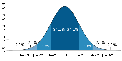
This is a question of statistical significance. To begin to answer this question, we need something to compare our results to. In statistics, that something is called a distribution. In this example, we need to know the distribution of cancer diagnoses in the population–in other words, we need to know how many cancer diagnoses we could reasonably expect to occur naturally in the absence of exposure to our chemical of interest. You have probably heard of the normal distribution or “bell curve.” Many biological measures follow a normal distribution. What this means is that if we take a measurement from every single person in the population, for example, height, and then plot it on a graph with the measure on the x-axis and the frequency at which that measure appears in the sample on the y-axis, we will get something that looks like this:
Assuming for this example that cancer diagnoses follow the same bell curve pattern, we now have a way of testing how certain we are that our results are not simply due to chance. In statistics, this is called a hypothesis test. Our hypothesis is that this chemical increases an exposed person’s risk of cancer. We want to determine how likely it is that our results are reflective of this association. To do this, we first assume the null hypothesis, which is that our results were observed purely by chance. When we test our hypothesis, our goal is to accept or reject this null hypothesis.
The steps to conducting a hypothesis test are as follows:
Identify the null and alternative hypotheses
Determine the appropriate test statistic and its distribution under the assumption that the null hypothesis is true
Decide what significance level you will use as your cut-off point for determining which hypothesis is acceptable (usually 95%)
Calculate the test statistic from the data to determine the p-value
Without getting into the calculations themselves, using the hypothetical sample above and assuming a normal distribution, the p-value is 0.2623. If we have selected the correct distribution for the data, this means that we could expect to see the observed result about 27% of the time purely by chance. Note that this is different from saying that we are 73% certain that our result is correct. P-values are only ever a measure of the probability of observing a value as or more extreme given that the null hypothesis is true (no true relationship between the chemical and cancer). In other words, they are a measure of how confident we are in the methods we have selected to analyze the data, rather than our confidence in the data themselves.
A confidence interval can be calculated in a similar manner, but it provides a range of values that could theoretically fall within a given significance level (also usually 95%). That is, the confidence interval tells us which values fall within the 95% significance level. You can think of this as a list of equally possible solutions given our data and the distribution we have chosen to compare them to. A narrow confidence interval indicates a higher level degree of “confidence” in the result because we have fewer possible solutions. A wide confidence interval indicates less certainty, because we have a wider range of values that could theoretically meet the significance threshold. If a confidence interval includes the number 1, then we cannot reject the null hypothesis (1 indicates a null effect). Confidence intervals are now generally preferred over p-values because they provide the reader with substantially more information about the level of certainty in the results.
One last takeaway is that p-values and confidence intervals only tell us about our degree of confidence in the study results, contingent on using a good design and the correct statistical measures and distributions; a significant p-value or narrow confidence interval does not necessarily mean that the association is causal, or even that an association truly exists at all. Remember, with a 95% significance level, the observation would still occur by chance 5% of the time! Likewise, just because a result does not meet the 95% threshold does not mean that we have proven there is no true association. If you are presenting scientific research to others, it is important to use language that does not inaccurately convey the results of the statistical analysis. Science relies on replication and reproducibility because we need many significant results to establish a true effect or association is present.
For a deeper dive into this topic, this article provides a good general introduction to p-values and significance testing.


Comments